Pourbaix Diagram for Iron
[1]:
import pyPourbaix as pb
Now that we have all the basics covered, we can get cracking with some more complicated stuff. Let’s finish off this tutorial line by creating a Pourbaix diagram for the iron-carbonate system. On top of the regular species required to plot the HER and OER, we will add crystalline iron, \(\text{Fe}^0(s)\), white rust, \(\text{Fe}(\text{OH})_2(s)\), maghemite, \(\text{Fe}_2\text{O}_3(s)\) and magnetite, \(\text{Fe}_3\text{O}_4(s)\) to our species database:
[2]:
species = ('H|+1|,      state=aq,   dGf=0,              dHf=0,              Sm=0',
           'H2,         state=g,    dGf=0,              dHf=0,              Sm=0',
           'e|-1|,      state=e,    dGf=0,              dHf=0,              Sm=0',
           'H2O,        state=l,    dGf=-2.37140E+05,   dHf=-2.85830E+05,   Sm=69.95',
           'O2,         state=g,    dGf=0,              dHf=0,              Sm=205.137',
           'Fe,         state=s,    dGf=0,              dHf=0,              Sm=27.1',
           'Fe(OH)2,    state=s,    dGf=-494.89E+03,    dHf=-583.4E+03,     Sm=84.0',
           'Fe2O3,      state=s,    dGf=-744.45E+03,    dHf=-826.3E+03,     Sm=87.4',
           'Fe3O4,      state=s,    dGf=-1012.72E+03,   dHf=-1115.8E+03,    Sm=145.9'
           )
In contrast to the other sample cases seen thus far, iron features aqueous species with two different oxidations states, the ferric ion \(\text{Fe}^{+2}\) and the ferrous ion \(\text{Fe}^{+3}\). We will also include a hydrolysed form of the ferric ion, \(\text{FeOH}^+\):
[3]:
species = ('H|+1|,      state=aq,   dGf=0,              dHf=0,              Sm=0',
           'H2,         state=g,    dGf=0,              dHf=0,              Sm=0',
           'e|-1|,      state=e,    dGf=0,              dHf=0,              Sm=0',
           'H2O,        state=l,    dGf=-2.37140E+05,   dHf=-2.85830E+05,   Sm=69.95',
           'O2,         state=g,    dGf=0,              dHf=0,              Sm=205.137',
           'Fe,         state=s,    dGf=0,              dHf=0,              Sm=27.1',
           'Fe(OH)2,    state=s,    dGf=-494.89E+03,    dHf=-583.4E+03,     Sm=84.0',
           'Fe2O3,      state=s,    dGf=-744.45E+03,    dHf=-826.3E+03,     Sm=87.4',
           'Fe3O4,      state=s,    dGf=-1012.72E+03,   dHf=-1115.8E+03,    Sm=145.9',
           'Fe|+2|,     state=aq,   dGf=-91504,         dHf=-92257,         Sm=-105.855',
           'Fe|+3|,     state=aq,   dGf=-16.23E+03,     dHf=-50.1E+03,      Sm=-282.4',
           'FeOH|+1|,   state=aq,   dGf=-274.00E+03,    dHf=-321.50E+03,    Sm=-29.6',
           )

reactions = ('2H|+1| + 2e|-1| -> H2',
             'O2 + 4H|+1| + 4e|-1| -> 2H2O',
             'Fe -> Fe|+2| + 2e|-1|',
             'Fe|+2| -> Fe|+3| + e|-1|',
             'Fe|+2| + 2H2O -> Fe(OH)2 + 2H|+1|',
             '3Fe|+2| + 4H2O -> Fe3O4 + 8H|+1| + 2e|-1|',
             'Fe + 2H2O -> Fe(OH)2 + 2H|+1| + 2e|-1|',
             '3Fe(OH)2 -> Fe3O4 + 2H2O + 2H|+1| + 2e|-1|',
             '2Fe3O4 + H2O -> 3Fe2O3 + 2H|+1| + 2e|-1|',
             'Fe|+3| + 1.5H2O -> 0.5Fe2O3 + 3H|+1|',
             'Fe|+2| + 1.5H2O -> 0.5Fe2O3 + 3H|+1| + e|-1|'
             )

db = pb.Database.from_default(species)
After adding a bunch of rections and inspecting our created database of species, it looks like we are good to go:
[4]:
print(db)
----------------------------Database----------------------------
Species              dGf             dHf              Sm
----------------------------------------------------------------
H|+1|                0.0             0.0             0.0
H2                   0.0             0.0             0.0
e|-1|                0.0             0.0             0.0
H2O             -237140.0       -285830.0          69.95
O2                   0.0             0.0         205.137
Fe                   0.0             0.0            27.1
Fe(OH)2         -494890.0       -583400.0           84.0
Fe2O3           -744450.0       -826300.0           87.4
Fe3O4           -1012720.0      -1115800.0         145.9
Fe|+2|          -91504.0        -92257.0        -105.855
Fe|+3|          -16230.0        -50100.0          -282.4
FeOH|+1|        -274000.0       -321500.0          -29.6
----------------------------------------------------------------
Skipping over the previously introduced pyPorbaix functionality, we have created a reactive system called Fe_system at default temperature and pressure, some pH and potential limits with respect to the SHE:
[5]:
Fe_system = pb.System()
Fe_system.set_database(db)
Fe_system.pHs = (0, 14)
Fe_system.electrode_potentials = (-1, 2)
Fe_system.reference_electrode = ("SHE" ,0.00)
Naturally, the system requires hydrogen, oxygen and iron to be amongst the elements from which species are to be plotted. For now, we can set the activity of all aqueous species to an arbitrary value of \(\{\text{Fe}\}_{\text{aq}} =1\times10^{-6}\) M.
[6]:
Fe_system.add_elements(["O","H","Fe"])
Fe_system.set_aqueous_activity("Fe",1e-6)
Fe_system.add_reactions(reactions)
The latter Fe_system will be our base-case before adding the remaining carbonate species and reactions. Before we proceed, lets quickly check whether the potential-pH diagram excluding the carbonate speices is correct.
[7]:
Fe_diagram = pb.PourbaixDiagram(Fe_system)
Fe_diagram.solve()
Fe_diagram.show(backend='matplotlib')

Looking good!
The major difference between a pure iron and a mixed iron-carbonate pourbaix diagram is the presence of siderite, \(\text{FeCO}_3(s)\) at circumneutral pH. To account for its formation, we will have to slightly modify the list of species and chemical reactions, adding aqueous \(\text{CO}_2(aq)\), the carbonate \(\text{HCO}_3^-\) and bicarbonate \(\text{CO}_3^{-1}\) anion, siderite, \(\text{FeCO}_3(s)\), as well as all iron-to-siderite transitions. Other reactions including the transition of e.g. \(\text{Fe}^{+2}\) to white rust are omitted.
[8]:
species = ('H|+1|,      state=aq,   dGf=0,              dHf=0,              Sm=0',
           'H2,         state=g,    dGf=0,              dHf=0,              Sm=0',
           'e|-1|,      state=e,    dGf=0,              dHf=0,              Sm=0',
           'H2O,        state=l,    dGf=-2.37140E+05,   dHf=-2.85830E+05,   Sm=69.95',
           'O2,         state=g,    dGf=0,              dHf=0,              Sm=205.137',
           'Fe,         state=s,    dGf=0,              dHf=0,              Sm=27.1',
           'Fe(OH)2,    state=s,    dGf=-494.89E+03,    dHf=-583.4E+03,     Sm=84.0',
           'Fe2O3,      state=s,    dGf=-744.45E+03,    dHf=-826.3E+03,     Sm=87.4',
           'Fe3O4,      state=s,    dGf=-1012.72E+03,   dHf=-1115.8E+03,    Sm=145.9',
           'Fe|+2|,     state=aq,   dGf=-91504,         dHf=-92257,         Sm=-105.855',
           'Fe|+3|,     state=aq,   dGf=-16.23E+03,     dHf=-50.1E+03,      Sm=-282.4',
           'FeOH|+1|,   state=aq,   dGf=-274.00E+03,    dHf=-321.50E+03,    Sm=-29.6',
           'CO2,        state=aq,   dGf=-385.970e+03,   dHf=-413.260e+03,   Sm=119.360',
           'HCO3|-1|,   state=aq,   dGf=-586.845e+03,   dHf=-689.930e+03,   Sm=98.400',
           'CO3|-2|,    state=aq,   dGf=-527.900e+03,   dHf=-675.230e+03,   Sm=50.000',
           'FeCO3,      state=s,    dGf=-679.557e+03,   dHf=-752.609e+03,   Sm=95.537'
           )

reactions = ('2H|+1| + 2e|-1| -> H2',
             'O2 + 4H|+1| + 4e|-1| -> 2H2O',
             'Fe -> Fe|+2| + 2e|-1|',
             'Fe|+2| -> Fe|+3| + e|-1|',
             'Fe + 2H2O -> Fe(OH)2 + 2H|+1| + 2e|-1|',
             '3Fe(OH)2 -> Fe3O4 + 2H2O + 2H|+1| + 2e|-1|',
             '2Fe3O4 + H2O -> 3Fe2O3 + 2H|+1| + 2e|-1|',
             'Fe|+2| + 1.5H2O -> 0.5Fe2O3 + 3H|+1| + e|-1|',
             'Fe|+3| + 1.5H2O -> 0.5Fe2O3 + 3H|+1|',
             'Fe|+2| + HCO3|-1| -> FeCO3 + H|+1|',
             '2FeCO3 + 3H2O -> Fe2O3 + 2HCO3|-1| + 4H|+1| + 2e|-1|',
             '3FeCO3 + 4H2O -> Fe3O4 + 3HCO3|-1| + 5H|+1| + 2e|-1|',
             'FeCO3 + 2H2O -> Fe(OH)2 + H|+1| + HCO3|-1|',
             'Fe + HCO3|-1| -> FeCO3 + H|+1| + 2e|-1|'
             )

db = pb.Database.from_default(species)
We will proceed and create an entirely new reactive system called Fe_C_system, load the new database and reactions, but keep all remaining properties the same:
[9]:
Fe_C_system = pb.System()
Fe_C_system.set_database(db)
Fe_C_system.pHs = (0, 14)
Fe_C_system.electrode_potentials = (-2, 2)
Fe_C_system.reference_electrode = ("SHE" ,0.00)
As we now have several aqueous species aassociated with different elements included in the diagram, we will have to set the aqueous activity of both iron and carbon. For now, they are set to \(\{\text{Fe}\}_{\text{aq}} = 1\times10^{-5}\) M and \(\{\text{C}\}_{\text{aq}} =1\times10^{-2}\) M.
[10]:
Fe_C_system.add_elements(["O","H","Fe","C"])
Fe_C_system.set_aqueous_activity("Fe",1e-5)
Fe_C_system.set_aqueous_activity("C",1e-2)
Fe_C_system.add_reactions(reactions)
After a quick inspection of the rective system,
[11]:
print(Fe_C_system)
-----------------------------System-----------------------------
Temperature : 298.15, Pressure : 1.0
----------------------------------------------------------------
        1.0H₂ ⇄ 2.0H⁺¹ + 2.0e⁻¹
        2.0H₂O ⇄ 1.0O₂ + 4.0H⁺¹ + 4.0e⁻¹
        1.0Fe⁺² + 2.0e⁻¹ ⇄ 1.0Fe
        1.0Fe⁺³ + 1.0e⁻¹ ⇄ 1.0Fe⁺²
        1.0Fe(OH)₂ + 2.0H⁺¹ + 2.0e⁻¹ ⇄ 1.0Fe + 2.0H₂O
        1.0Fe₃O₄ + 2.0H₂O + 2.0H⁺¹ + 2.0e⁻¹ ⇄ 3.0Fe(OH)₂
        3.0Fe₂O₃ + 2.0H⁺¹ + 2.0e⁻¹ ⇄ 2.0Fe₃O₄ + 1.0H₂O
        0.5Fe₂O₃ + 3.0H⁺¹ + 1.0e⁻¹ ⇄ 1.0Fe⁺² + 1.5H₂O
        0.5Fe₂O₃ + 3.0H⁺¹ ⇄ 1.0Fe⁺³ + 1.5H₂O
        1.0FeCO₃ + 1.0H⁺¹ ⇄ 1.0Fe⁺² + 1.0HCO₃⁻¹
        1.0Fe₂O₃ + 2.0HCO₃⁻¹ + 4.0H⁺¹ + 2.0e⁻¹ ⇄ 2.0FeCO₃ + 3.0H₂O
        1.0Fe₃O₄ + 3.0HCO₃⁻¹ + 5.0H⁺¹ + 2.0e⁻¹ ⇄ 3.0FeCO₃ + 4.0H₂O
        1.0Fe(OH)₂ + 1.0H⁺¹ + 1.0HCO₃⁻¹ ⇄ 1.0FeCO₃ + 2.0H₂O
        1.0FeCO₃ + 1.0H⁺¹ + 2.0e⁻¹ ⇄ 1.0Fe + 1.0HCO₃⁻¹
----------------------------------------------------------------
we are good to go, generating the final iron-carbonate Pourbaix diagram:
[12]:
Fe_C_diagram = pb.PourbaixDiagram(Fe_C_system)
Fe_C_diagram.solve()
Fe_C_diagram.show(backend='matplotlib')
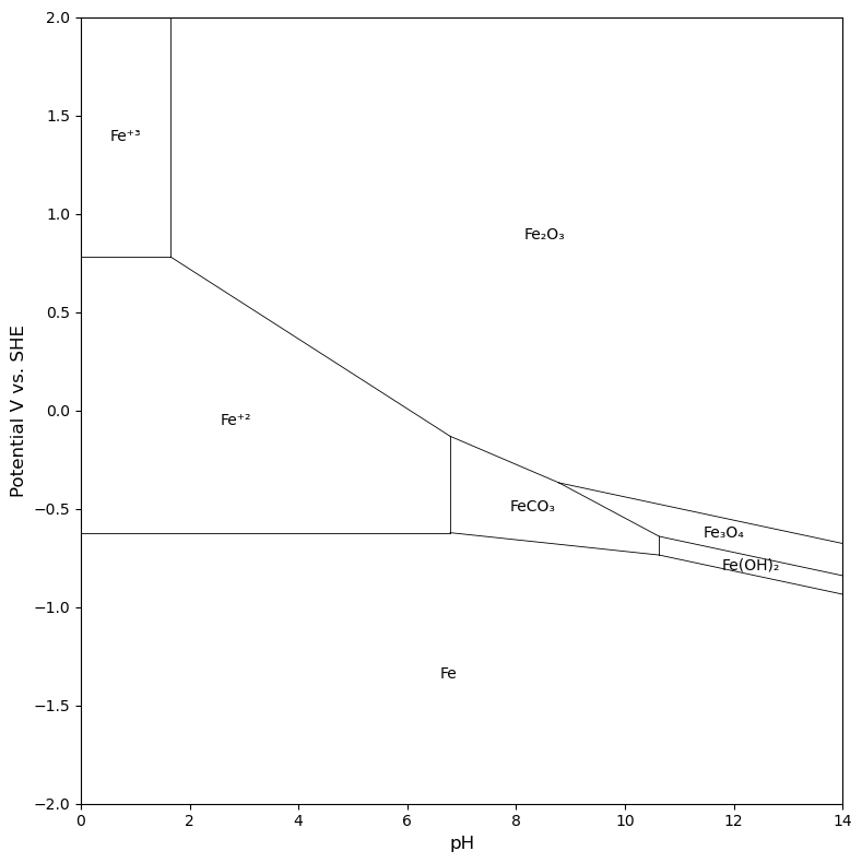
Interacting with the final diagram
After including so many phases in the diagram, it may be easy to loose track which ones actually feature a region of stability in across the slected potential and pH space and which ones don’t. We can easily check this by running the command Fe_C_diagram.get_stable_phases():
[19]:
Fe_C_diagram.get_stable_phases()
[19]:
dict_keys(['Fe', 'Fe⁺²', 'Fe⁺³', 'Fe(OH)₂', 'Fe₃O₄', 'Fe₂O₃', 'FeCO₃'])
Here we go, it appears that a total of 7 phases are stable in the given space of physiochemical conditions selected. Of course, this excludes the phases needed to vary the pH and potential in the diagram, e.g. the \(\text{H}^+\) cations. Suppose we are interested in the phase that is stable at a given (pH,E) coordinate. Nothing easier than that, let’s inspect the phase stable at pH = 4 and open circuit conditions using Fe_diagram.get_stable_phase_at(pH=4, potential=0):
[20]:
print(f'The stable phase at pH = 4 and E = 0 is {Fe_diagram.get_stable_phase_at(pH=4, potential=0)}')
The stable phase at pH = 4 and E = 0 is Fe⁺²
A quick comparison with the generated Pourbaix diagram will tell us that the stable phase at pH = 4 and E = 0 V vs SHE is indeed \(\text{Fe}^{2+}\). How about the one just above at a potential E = 1 V vs. SHE?
[21]:
print(f'The stable phase at pH = 4 and E = 1 is {Fe_diagram.get_stable_phase_at(pH=4, potential=1)}')
The stable phase at pH = 4 and E = 1 is Fe₂O₃
Shifting the potential by 1 V in positive y-direction, we have crossed the reaction line of \(\text{Fe}^{2+}\) to \(\text{Fe}_2\text{O}_3(s)\) oxidation. Correspondingly, the stable phase at coordinates (4,1) is \(\text{Fe}_2\text{O}_3(s)\).